Animate overdose

Here,

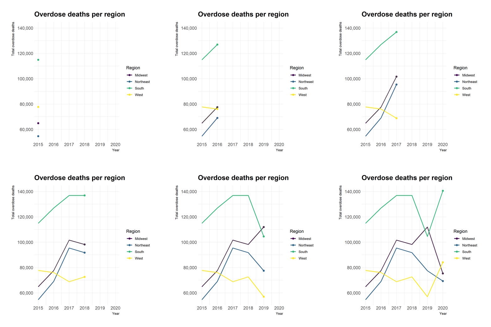
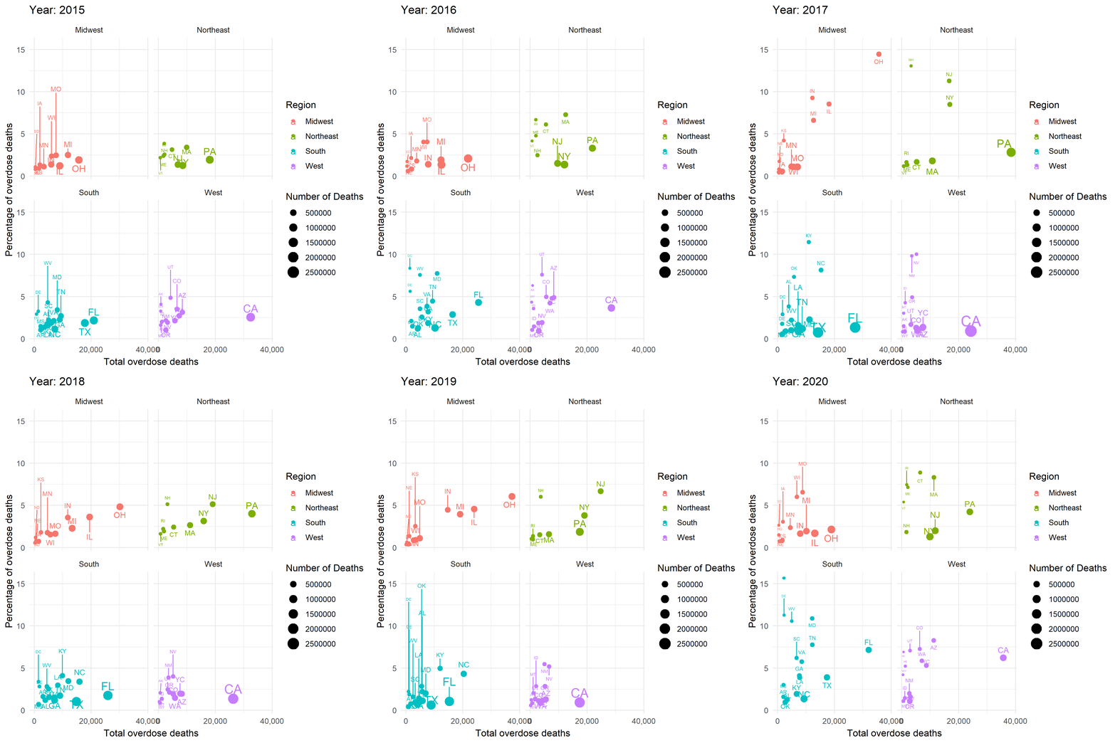
I animate the evolution of overdose deaths in the US from 2015 to 2020. The data was fetched from CDC's open data warehouse. Scroll down to check the code I used to produce this.

Here are the gifs that we produced with the procedure. Note that, region wise, overdose deaths do not seem to follow a pattern. We can see how Covid affected mostly southern states. And that, luckily, the Midwest saw their overall overdose deaths decrease. This is not entirely good news. The Ohio state, as shown in the second animation, has had high percentages and total count of overdose deaths during the pandemic.

Per region animation

Per state animation

Learn More

Use R

# Set working directory
setwd(paste0("C:/Users/", Sys.info()[["user"]], "/Documents/Prototypes/Animate_overdose"))

# Load the data
`Overdose_death_count_US_2015-2020` <- read.csv("data/VSRR_Provisional_Drug_Overdose_Death_Counts.csv")

# Load libraries
library(tidyverse)
library(gganimate)
library(ggrepel)
library(hrbrthemes)
library(viridis)
  # Load library to render gifs.
library(gifski)

# Filter data. Select values. Pivot. Add Region variable.
death_count_US <- `Overdose_death_count_US_2015-2020` %>%
  filter(Indicator == c("Number of Drug Overdose Deaths", "Number of Deaths")) %>%
  select(State, Year, Month, Period, Indicator, Data.Value) %>%
  pivot_wider(names_from = Indicator, values_from = Data.Value) %>%
  # Create a proper division of states.  
  mutate(
    Region = case_when(
      State %in% c("PA", "NY", "VT", "NH", "ME", "MA", "RI", "CT", "NJ", "RI") ~ "Northeast",
      State %in% c("OH", "MI", "IN", "IL", "WI", "IA", "MN", "MO", "KS", "SD", "NE", "ND") ~ "Midwest",
      State %in% c("DC", "DE", "MD", "VA", "WV", "NC", "SC", "KY", "TN", "GA", "FL", "AL", "MS", "LA", "AR", "OK", "TX") ~ "South",
      State %in% c("YC", "NM", "CO", "AZ", "UT", "WY", "MT", "ID", "CA", "NV", "OR", "WA", "AK", "HI") ~ "West",
      State %in% c("US") ~ "US"
    ))

# Summarize per region
death_count_region <- death_count_US %>%
  group_by(Region, Year) %>%
  summarise(.data = ., across(c("Number of Drug Overdose Deaths", "Number of Deaths"), sum, na.rm = TRUE))

# Summarize per state
death_count_state <- death_count_US %>%
  group_by(Region, State, Year) %>%
  summarise(.data = ., across(c("Number of Drug Overdose Deaths", "Number of Deaths"), sum, na.rm = TRUE)) %>%
  mutate(`Overdose deaths percentage` = `Number of Drug Overdose Deaths` / `Number of Deaths` * 100)

# Store animation object. Region data
store_animation_region <- ggplot(data = death_count_region %>% filter(Region != "US"),
       aes(x = Year, y = `Number of Drug Overdose Deaths`, color = Region)) +
  labs(title = "Overdose deaths per region", y = "Total overdose deaths") +
  geom_point(size = 2) +
  geom_line(size = 1) +
  scale_y_continuous(labels = scales::comma, breaks = scales::pretty_breaks(n = 5)) +
  theme_ipsum() +
  scale_color_viridis(discrete = TRUE) +
  # Animate plot.
  transition_reveal(Year) +
  enter_fade() +
  exit_fade()

# Store animation object. State data.
store_animation_state <- ggplot(data = death_count_state %>% filter(State != "US"),
       aes(x = `Number of Drug Overdose Deaths`, y = `Overdose deaths percentage`,
           color = Region, size = `Number of Deaths`, label = State)) +
  labs(title = "Year: {frame_time}", y = 'Percentage of overdose deaths', x = 'Total overdose deaths') +
  geom_point() +
  theme_minimal() +
  scale_x_continuous(labels = scales::comma, breaks = scales::pretty_breaks(n = 2)) +
  # Separate data points from names.  
  geom_text_repel(direction = "y", seed = 123, box.padding = 0.4) + # Set non-random seed in text repel
  # Animate plot
  transition_time(Year) +
  ease_aes('linear') +
  # Create 1 plot per region
  facet_wrap(~Region) +
  enter_fade() +
  exit_fade()

# Save animations as .gif
# Save region animation
anim_save(filename = "animations/drug_overdose_animation_region_lq.gif", animation = store_animation_region,
          units = "in", height = 6, width = 6, res = 300, fps = 60, nframes = 300, duration = 4)
# Save state animation
anim_save(filename = "animations/drug_overdose_animation_state_lq.gif", animation = store_animation_state,
          units = "in", height = 6, width = 6, res = 300, fps = 60, nframes = 300, duration = 12)